In this article, I’m going to cover the basics of SciPy that can help you get started with it. I am going to cover important sub-packages of SciPy with practical examples. Also in the end we will discuss some important functions from the python SciPy library.
SciPy or scientific computation or programming deals with scientific and mathematical computations which is a fundamental python package that helps you to drill down the computation portion of data analysis. The scientific operation includes arrays, matrices, Integration, Differential Equation Solving, Statistics, and many more which are not part of python inbuilt operations. So, all the scientific calculations and programming are done by using SciPy at an advanced level.
Table of content
By the end of this reading, you’ll be able to understand,
- What is SciPy and Why SciPy is needed?
- The characteristics of SciPy
- SciPy and NumPy
- Different sub-packages of SciPy
- SciPy Sub-Packages with a practical example
- Some Special SciPy Functions
- Conclusion
What Is SciPy And Why SciPy Is Needed?
SciPy is an extension of python NumPy library. SciPy has built-in packages that help in handling the scientific domains. SciPy can be used to work with the following scientific domains,
- Mathematical equations
- Image science
- Spatial data
- Statistics
- Optimization
- Signal processing
- Platform integration
The Main Characteristics Of SciPy
Let’s understand what makes SciPy such a great library for Scientific computing.
- SciPy has Built-in mathematical libraries and functions for complex scientific computation.
- SciPy High-level commands make data manipulation and visualization easy.
- As SciPy is built on top of NumPy the data processing is faster.
- SciPy integrates very well with multiple systems and environments.
- SciPy comes with a large set of sub-packages for different scientific domains.
- SciPy’s developer-friendly functions make scientific application development easy for developers.
NumPy And SciPy
Both NumPy and SciPy used for mathematical and numerical analysis.
NumPy contains array data that can perform operations like sorting, indexing, slicing, etc, While SciPy consists of all the numerical codes.
If we are doing scientific operations with linear algebra and other mathematical functions though NumPy can solve the problems SciPy is the best-suited option for these.
Different Sub-Packages Of SciPy
Now let’s see some of the most popular packages of SciPy that are widely used for scientific computing across different domains.
| Sub-Package Name | Description |
|---|---|
| scipy.cluster | It is used for Clustering algorithms & is used to vector quantization/ Kmeans. |
| scipy.constants | It Is used for the physical and mathematical constants. |
| scipy.fftpack | It is used for doing a Fourier transform. |
| scipy.integrate | It is used for Integration routines |
| scipy.interpolation | It is used for Interpolation |
| scipy.linalg | It is used for linear algebra routine. |
| scipy.io | It is used for data input and output. |
| scipy.ndimage | It is used for the n-dimension image. |
| scipy.odr | It is used for Orthogonal distance regression. |
| scipy.optimize | It is used for optimization. |
| scipy.signal | It is used in signal processing. |
| scipy.sparse | It is used for Sparse matrices and associated routines. |
| scipy.spatial | It is used for Spatial data structures and algorithms. |
| scipy.special | It is used for Special Function. |
| scipy.stats | It is used for Statistics. |
| scipy.weaves | It is used for It is a tool for writing. |
SciPy Sub-Packages With a Practical Example
Now Let’s understand a few Important of these sub-packages with a practical example. You can try the below code yourself on your own computer. If you want all the code you can find it on my GitHub repository.
SciPy Cluster (scipy.cluster):
Clustering is the way of dividing or classifying the datasets into groups. Suppose in a class the students are grouped based on the marks obtained. In clustering, the K-means clustering is a process of finding clusters and cluster centers in a set of unlabeled data.
import numpy as np
from scipy.cluster.vq import kmeans, vq, whiten
from numpy import vstack, array
from numpy.random import rand

#data generation
data = vstack((rand(50,3) + array([.3,.3,.3]), rand(50,3)))

#whitening of data
data_w = whiten(data)

#computing k-means with k=3 (2 cluster)
centroid = kmeans(data_w,3)
print(centroid)

Output:
(array([[2.76362046, 2.52153412, 1.71175   ],
       [1.22771333, 1.18327701, 1.42998892],
       [2.1281064 , 2.54411162, 3.18968839]]), 1.160723810720625)
SciPy Constants (SciPy.constants) :
SciPy constant package has a good amount of mathematical and physical constants.
## Scipy Constant package
from scipy.constants import pi
print(pi)
Output:3.141592653589793

import scipy.constants
result = scipy.constants.physical_constants["alpha particle mass"]
print(result)
Output: (6.6446573357e-27, 'kg', 2e-36)
Here are some of the constants we can work with using Python SciPy.Constant package.
Mathematical Constant: pi, golden,
Physical Constants: c – Speed of light in vacuum, speed_of_light – Speed of light in vacuum, h – Planck constant, G – Newton’s gravitational constant, e – Elementary charge, R – Molar gas constant, Avogadro – Avogadro constant, k – Boltzmann constant, electron_mass(OR) m_e – Electronic mass, proton_mass (OR) m_p – Proton mass, neutron_mass(OR)m_n – Neutron mass
Units Constants: milli, micro, kilo
SciPy FFTPack (scipy.fftpack):
FFTP is a sub package of SciPy to calculate Fourier Transformation which is calculated on a time-domain signal to check its behavior in the frequency domain.
#importing fft and inverse fft functions from fftpackage
from scipy.fftpack import fft
import numpy as np
#creating an array with random numbers
arr = np.array([2.0, 4.0, 2.0, -2.0, 2.5])
#applying the fft function
arr_fft = fft(arr)
print(arr_fft)
Output: [ 8.5       -0.j          4.00861046-3.77772578j -3.25861046+2.92254819j
 -3.25861046-2.92254819j  4.00861046+3.77772578j]
SciPy Interpolation (scipy.interpolate):
Interpolation is a sub package of SciPy for finding new data points within a set of known data points.
#interplation scipy sub package
import numpy as np
from scipy import interpolate
import matplotlib.pyplot as plt

x = np.linspace(1, 5, 13)
y = np.cos(x**3/4+5)
print(x,y)
Output: [1.         1.33333333 1.66666667 2.         2.33333333 2.66666667
 3.         3.33333333 3.66666667 4.         4.33333333 4.66666667
 5.        ] [ 0.51208548  0.77086859  0.99210038  0.75390225 -0.31641156 -0.95049765
  0.68487032 -0.12178922  0.04529897 -0.54772926  0.97806189  0.53311419
  0.12138441]

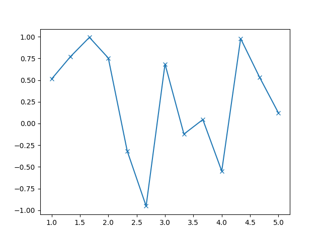
plt.plot(x, y, marker="x")
plt.show()
Output: see the graph below.
SciPy Linear Algebra (scipy.linalg):
SciPy has very fast linear algebra capabilities. scipy.linalg contains all the functions that are present in NumPy.linalg but it also has some additional functions.
#import the scipy and numpy packages
from scipy import linalg
import numpy as np

#Declaring the numpy arrays
arr1 = np.array([[3, 2, 0], [1, -1, 0], [0, 5, 1]])
arr2 = np.array([2, 4, -1])

#Passing the values to the solve function
x = linalg.solve(arr1, arr2)

#printing the result array
print(x)
Output: [ 2. -2.  9.]
Finding a Determinant
from scipy import linalg
import numpy as np
Arr = np.array([[1,2],[3,4]])
x = linalg.det(Arr)
print(x)
OutPut: -2.0
Calculating an inverse of an matrix
#Calculate the Inverse of a matrix
arr1 = np.array([[3, 2, 0], [1, -1, 0], [0, 5, 1]])
arr_inverse = linalg.inv(arr1)
print(arr_inverse)
Output: [[ 0.2  0.4  0. ]
 [ 0.2 -0.6  0. ]
 [-1.   3.   1. ]]
With the help of scipy.linalg we can solve the eigenvalue-eigenvector problem which is one of the most commonly in linear algebra operations. Check below code to find Eigenvalues (λ) and the corresponding Eigenvectors (v) of a square matrix (A) by considering the relation − Av = λv
Arr = np.array([[1,2],[3,4]])
#Passing the values to the eig function
l, v = linalg.eig(Arr)
#printing the result for eigen values
print(l)
#printing the result for eigen vectors
print(v)
Output: [-0.37228132+0.j  5.37228132+0.j]
[[-0.82456484 -0.41597356]
 [ 0.56576746 -0.90937671]]
SciPy Input and Output (scipy.io):
Scipy input out sub-package provides a different set of functions to work with a different set of file formats Check the code below.
import scipy.io as sio
#Saving a mat file
vect = np.arange(10)
sio.savemat('array.mat', {'vect':vect})
#loading a file
mat_file_content = sio.loadmat('array.mat')
print(mat_file_content)

Output: {'__header__': b'MATLAB 5.0 MAT-file Platform: posix, Created on: Sat Aug 15 10:35:20 2020', '__version__': '1.0', '__globals__': [], 'vect': array([[0, 1, 2, 3, 4, 5, 6, 7, 8, 9]])}
SciPy Ndimage (scipy.ndimage):
SciPy Ndimage package provide general image processing and analysis functions.
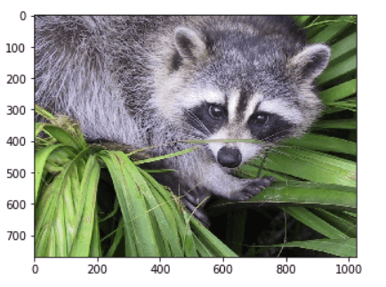
from scipy import misc
fi = misc.face()
misc.imsave('face.jpg', fi)
import matplotlib.pyplot as plt
plt.imshow(fi)
plt.show()

#second image
flip_ud_face = np.flipud(face)
import matplotlib.pyplot as plt
plt.imshow(flip_ud_face)
plt.show()

#third image
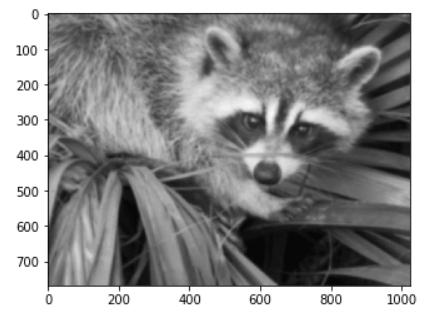
blurred_image = ndimage.gaussian_filter(face, sigma=4)
import matplotlib.pyplot as plt
plt.imshow(blurred_face)
plt.show()

#fourth image
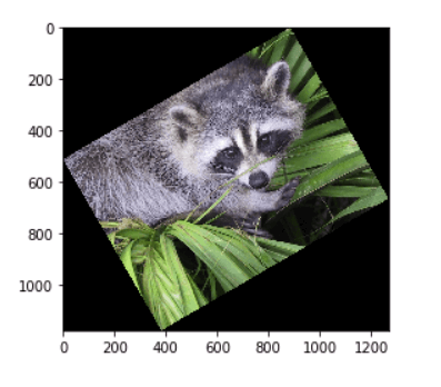
rotate_face = ndimage.rotate(face, 30) #rotating the image 30 degree
import matplotlib.pyplot as plt
plt.imshow(rotate_face)
plt.show()

Output: See the below images for all output. (YOU NEED TO RUN EACH CODE SEPARATELY) 
FOURTH OUTPUT IMAGE 
THIRD OUTPUT IMAGE 
SECOND OUTPUT IMAGE 
FIRST OUTPUT IMAGE
SciPy Optimize (scipy.optimize):
The SciPy Optimize packages provide different optimization algorithms. It contains the following aspects,
- Global optimization routines(brute-force, anneal(), basinhopping())
- With the help of various algorithms (BFGS, Nelders-Mead simplex, Newton Conjugate Gradient, COBLYA) it allows unconstrained and constrained minimization of the multivariate scalar functions(minimize())
- Least-squares minimization algorithms(leastsq() and curve fit()
- Scalar univariate function minimizers (minimizer_scalar() and root finders newton())
Nelder–Mead Simplex Algorithm:
import numpy as np
from scipy.optimize import minimize
def rosen_f(x):
a = np.array([1.3, 0.7, 0.8, 1.9, 1.2])
res = minimize(rosen_f, a, method='nelder-mead')
print(res.a)
Output: [7.93700741e+54  -5.41692163e+53  6.28769150e+53  1.38050484e+55  -4.14751333e+54]
Some Special SciPy Functions
Now let’s understand some most common and special SciPy functions. These functions are also called universal functions.
#Cubic root function
from scipy.special import cbrt
result = cbrt([4, 9, 0.1234])
print(result)
Output: [1.58740105 2.08008382 0.4978575 ]

#exponential function
from scipy.special import exp10
result = exp10([4,16])
print(result)
Output: [1.e+04 1.e+16]

#Relative Error Exponential Function
from scipy.special import exprel
result = exprel([-0.25, -0.1, 0, 0.1, 0.25])
print(result)
Output: [0.88479687 0.95162582 1.         1.05170918 1.13610167]

#Log Sum Exponential Function
from scipy.special import logsumexp
import numpy as np
arr = np.arange(20)
result = logsumexp(arr)
print(result)
Output:19.458675143325927

#Lambert Function
from scipy.special import lambertw
w = lambertw(1)
print(w)
print(w * np.exp(w))
Output: (0.5671432904097838+0j)
(1+0j)

#Permutations and Combinations Function
from scipy.special import comb
result = comb(15, 5, exact = False, repetition = True)
print(result)
Output: 11628.0

#permutation
from scipy.special import perm
result = perm(15, 9, exact = True)
print(result)
Output:1816214400

#Gamma fuction
from scipy.special import gamma
result = gamma([1, 1.5, 2, 7])
print(result)
Output: [  1.           0.88622693   1.         720.        ]
Conclusion
After finishing this blog post, I hope that you have a fair understanding of Scientific computing using the SciPy library of python. There is a lot of things that we can do using SciPy. You can always refer to the SciPy documentation for more details. Proving the link below.
SciPy Documentation: https://docs.scipy.org/doc/scipy/reference/
Thank you! Happy Learning ????
